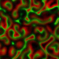
 Fig 4. Two populations showing predator front formation. +--+------------------+ |C0|1.5 _2e_5 _0.0001| | |0.5 0.0001 _1e_5| +--+------------------+ |M0|1 1 | +--+------------------+ |
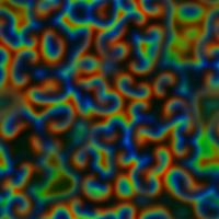 Fig 7. Three populations and curved fronts. +--+-----------------------------------------+ |C0| 1.53 _0.0980392 _0.980392 _1.02| | | 1.02 0.980392 _0.0980392 _1.02| | |0.490196 0.980392 0.980392 _0.0980392| +--+-----------------------------------------+ |M0|0.5 0.5 1 | +--+-----------------------------------------+ |
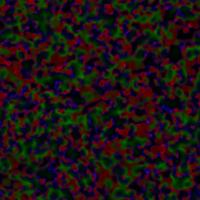 Fig 8. Light formation of spirals for one migration list +--+---------------------------------------+ |C0| 1.06121 _0.0942322 _0.773033 0.743015| | |0.714163 1.02 _0.106121 _1.14869| | | 1.5769 _0.980392 1.02 _0.114869| +--+---------------------------------------+ |M0|0.5 1 0.1 | +--+---------------------------------------+ |
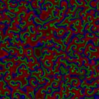 Fig 9. Well formed spirals for another migration list +--+---------------------------------------+ |C0| 1.06121 _0.0942322 _0.773033 0.743015| | |0.714163 1.02 _0.106121 _1.14869| | | 1.5769 _0.980392 1.02 _0.114869| +--+---------------------------------------+ |M0|1 0.5 1 | +--+---------------------------------------+ |
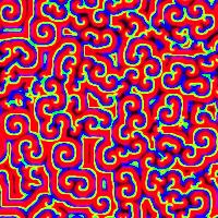 Fig 10. Very distinct spirals for one choice of upper bound. +--+------------------------+ |C0|1.6 _4e_6 _3e_5 1e_5| | |1.4 0.0001 _2e_5 _0.0003| | |0.7 0 5e_5 _1e_5| +--+------------------------+ |M0|1 1 1 | +--+------------------------+ |
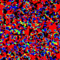 Fig 11. Less organized behavior for a higher upper bound. +--+------------------------+ |C0|1.6 _4e_6 _3e_5 1e_5| | |1.4 0.0001 _2e_5 _0.0003| | |0.7 0 5e_5 _1e_5| +--+------------------------+ |M0|1 1 1 | +--+------------------------+ |