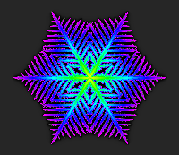
Growth
limited by
radius 100

Growth limited
by radius 200

Growth limited by radius 400
Auxiliary Materials for:
A Local Cellular Model for Snow Crystal Growth
by Cliff Reiter, May 2004
We consider a hexagonal array of real valued (nonnegative) cells with the following process for updating cells. We consider a cell to be solid ice if its value is greater than or equal to one. Then classify each cell at each step as either receptive or nonreceptive. Cells which are ice and their immediate neighbors are receptive. The updated value is the sum of two terms. The first term is the value of the receptive sites with a constant γ added; the second term is the average of the nonreceptive sites (with receptive sites contributing values of zero to the averages). The averaging consists of taking the average of the centervalue and the average of the immediate neighbors (with zeros as noted above). On some occasions we take weighted averages which will correspond to changing a parameter α. Ordinarily α=1. We usually begin with a single seed of value one with all other sites initialized at some background level β. Boundary conditions maintain the background level at a radius near the edge of the image.
First we consider tables showing how the growth appears on radius 100, 200 and 400 regions.
|
Growth limited by radius 100 |

Growth limited by radius 200 |

Growth limited by radius 400 |
 β=0 γ=1 |
 β=0.35 γ=0 |
 β=0.4 γ=0.001 |
 β=0.4 γ=0.002 |
 β=0.8 γ=0.002 |
 β=0.95 γ=0 |

Random 3 by 3 |
 α = 1, β varies, γ=0 |
 α = 1, β = 0.35, γ varies |
 α = 1, β = 0.4, γ varies |
 α varies 0 to 1, β = 0.4, γ = 0.0001 |
 α varies 2.4 to 2.7, β = 0.4, γ = 0.0001 |